Tutorials
Swalbe.jl is software that simulates the dynamics of a thin liquid film. At it's core is the lattice Boltzmann method (LBM) a mesoscale method that works based on particle distribtuion functions $f_i(\mathbf{x},t)$. To get a better understandig of both the LBM and the package we supply instructive simulations and discuss the content of the code.
Constant interface
A nice and easy way to check the consistency of a fluid mechanics solver is to prob the mass or density. Per continuity equation $\partial_t\rho + \nabla\cdot\mathbf{j} = 0$, we require that the local density $\rho$ can only change if there is a flux $\mathbf{j}$ (okay a divergence of a flux). In case of vanishing or constant flux $\nabla\cdot\mathbf{j} = 0$ the density has to be time independent and therefore $\partial_t \rho = 0$.
Thin film flows can be described with the same kind of equation
\[\partial_t h(\mathbf{x},t) + \nabla\left(M(h)\nabla p(\mathbf{x},t)\right) = 0. \]
The local height can only change with time if some pressure gradient
Having a vanshing pressure gradient the height $h(\mathbf{x},t)$ have to be constant independent of time. To check this we put together a small sample simulation that probes this.
using Swalbe # import the package
# Define the system size and parameters
sys = Swalbe.SysConst(Lx = 100, # 100 lattice units in x-direction
Ly = 100, # 100 lattice units in y-direction
Tmax = 1000) # LBM time loop runs for 1000 iterations
# Allocation of distribution functions, macroscopic variables and forces
fout, ftemp, feq, height, velx, vely, vsq, pressure, dgrad, Fx, Fy, slipx, slipy, h∇px, h∇py = Swalbe.Sys(sys, # Size
"CPU", # Where to run
false, # No fluctuations
Float64) # Num type
# Constant film thickness, or flat interface
height .= 1.0
# Compute the first equilibrium distribtuion function based on the initial conditions
Swalbe.equilibrium!(ftemp, height, velx, vely, vsq)
# Empty list to measure the total mass over time
mass = []
# To add the forcing due to a pressure gradient set true
pressure_gradient = false
# Start of the lattice Boltzmann time loop
for t in 1:sys.Tmax
# Fill the list
push!(mass,sum(height))
# Talks with us all t % tdump time sets
if t % sys.tdump == 0
println("Time step $t mass is $(round(sum(height), digits=3))")
end
if pressure_gradient
# The pressure computation
Swalbe.filmpressure!(pressure, height, dgrad, sys.γ, 1/9, sys.n, sys.m, sys.hmin, sys.hcrit)
# Pressure gradient
Swalbe.∇f!(h∇px, h∇py, pressure, dgrad, height)
# Slippage
Swalbe.slippage!(slipx, slipy, height, velx, vely, sys.δ, sys.μ)
# Summation of forces
Fx .= h∇px .+ slipx
Fy .= h∇py .+ slipy
end
# New equilibrium
Swalbe.equilibrium!(feq, height, velx, vely, vsq)
# Collision and streaming of distribution function
Swalbe.BGKandStream!(fout, feq, ftemp, Fx, Fy)
# Update of macroscopic quantities
Swalbe.moments!(height, velx, vely, fout)
# Next iteration
end
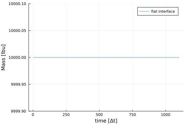
# Check if the mass is constant
using Plots
# Since h = 1 everywhere and the size 100 x 100 the mass has to be 100^2
plot(mass, xlabel="time [Δt]", ylabel="Mass [lbu]", label="flat interface", ylim=(100^2-0.1, 100^2+0.1))In fact this is a particular strength of the lattice Boltzmann method. Under the assumption that no forces are applied the mass is mathematically conserved. Which is shown in the lower plot
Dewetting of patterned a substrate
Next we take a look at substrates with a wettability gradient and show how to use an image or geometrical shapes to induce directed dewetting. Here we actually reuse the display simulation of the README.md. The idea is to use Youngs equation
\[\cos(\theta_{\text{eq}}) = \frac{\gamma_{sg} - \gamma_{sl}}{\gamma}, \]
where the $\gamma$'s are the three interfacial energies and $\theta_{\text{eq}}$ is the equilibrium contact angle to address the wettability of the substrate. Without problems it is possible to discretize $\theta_{\text{eq}}$ similar to the pressure or the film thickness and therefore effectively introduce a wettability gradient $\nabla \theta_{\text{eq}} \neq 0$. In the logo simulation what actually happens is that initial perturbations (ϵ * randn()) grow with time, leading to a film rupture and travelling rims. The ruptures are triggered in regions of high contact angle and the rims meet in regions of low contact angle (letters of the logo). There is a lot of theory involved and if you want to read up on it check out the review from Craster&Matar (paywall), especially section 5. Films driven by intermolecular forces.
But let's start again with some code, first with a triangle with lower wettability in the middle
using Swalbe

# Define the system size and parameters
sys = Swalbe.SysConst(Lx = 100,     # 100 lattice units in x-direction
                      Ly = 100,     # 100 lattice units in y-direction
                      n = 3,        # first disjoining pressure exponent
                      m = 2,        # second disjoining pressure exponent
                      Tmax = 1000)  # LBM time loop runs for 1000 iterations


# Allocation of distribution functions, macroscopic variables and forces
fout, ftemp, feq, height, velx, vely, vsq, pressure, dgrad, Fx, Fy, slipx, slipy, h∇px, h∇py = Swalbe.Sys(sys,      # Size
                                                                                                          "CPU",    # Where to run
                                                                                                          false,    # No fluctuations
                                                                                                          Float64)  # Num type
# Random (gaussian) perturbations put on top of a flat interface
ϵ = 0.001
height .= 1.0 .+ ϵ .* randn(sys.Lx, sys.Ly)
# The contact angle field
theta = fill(1/6, sys.Lx, sys.Ly)
# Lower contact angle in the middle of the substrate
Swalbe.trianglepattern(theta, 1/6, δₐ=-1/18)
# Compute the first equilibrium distribution function based on the initial conditions
Swalbe.equilibrium!(ftemp, height, velx, vely, vsq)
# Difference in total height with time
diff_h = []
# Start of the lattice Boltzmann time loop
for t in 1:sys.Tmax
    # Fill the difference list
    push!(diff_h, maximum(height) - minimum(height))
    # Talks with us all t % tdump time sets
    if t % sys.tdump == 0
        println("Time step $t mass is $(round(sum(height), digits=3))")
    end
    # The pressure computation
    Swalbe.filmpressure!(pressure, height, dgrad, sys.γ, theta, sys.n, sys.m, sys.hmin, sys.hcrit)
    # Pressure gradient
    Swalbe.∇f!(h∇px, h∇py, pressure, dgrad, height)
    # Slippage
    Swalbe.slippage!(slipx, slipy, height, velx, vely, sys.δ, sys.μ)
    # Summation of forces
    Fx .= -h∇px .- slipx
    Fy .= -h∇py .- slipy

    # New equilibrium
    Swalbe.equilibrium!(feq, height, velx, vely, vsq)
    # Collision and streaming of distribution function
    Swalbe.BGKandStream!(fout, feq, ftemp, Fx, Fy)
    # Update of macroscopic quantities
    Swalbe.moments!(height, velx, vely, fout)
    # Next iteration
end
# Another library for plotting and to my understanding actually the best you can do
using CairoMakie
# We are interested in the heatmap of the film thickness and the growth rate of the perturbation
let
	x1 = 1:1:sys.Tmax
	y2 = zeros(sys.Tmax)
	y2 .= diff_h
    fig = Figure(resolution = (960,450))

    ax1 = Axis(fig, xlabel = "time [Δt]", ylabel = "Δh [lbu]",xscale = log10, yscale = log10,xgridstyle=:dash, ygridstyle=:dash, xminorticksvisible = true,
        xminorticks = IntervalsBetween(9), yminorticksvisible = true,
        yminorticks = IntervalsBetween(9))
	leg = lines!(ax1, x1, y2, color = :navy)
	ax2 = Axis(fig,  aspect = 1, xlabel = "x [Δx]", ylabel = "y [Δx]")
    hmap = heatmap!(ax2, height, colormap = :viridis)
    cbar = Colorbar(fig, hmap, label = "thickness", ticksize=15, tickalign = 1, width = 15)
	fig[1,1] = ax1
    fig[1,2] = ax2
    fig[1,3] = cbar
    fig
end
Fluid is drained into regions of lower contact angle, therefore into in the triangle. The effect is the strongest around the vertices of the triangle. Since in principle this a dewetting instability with a well defined spectrum computable using the surface tension $\gamma$ and the disjoining pressure functional $\Pi(h)$. The result should look like the plot below

Of course you can and should play with the parameters ($\gamma$, $\delta$, $h_0$, ...) to get a physically correct simulation :wink:.
Droplet spreading in 1D
If a certain amount of liquid is placed on a surface, like a rain drop :droplet: hitting a plant leaf :fourleafclover: we observe a drop sticking to the leaf. The shape of the droplet is actually nature solving Young's law and finds an equilibrium shape which can be described by a simple macroscopic observable, the contact angle $\theta_{\text{eq}}$. There is of course more to it, for further reading check out Snoeijer & Andreotti We can recast this behavior with a simple and fast simulation.
In contrast to the two examples before we put the whole experiment into a function and just call the function. While this may seem overkill here it is in fact very useful. Instead of writing a script for every experiment, we simply write a function and loop through function arguments. Making it very convenient to perform phase space scans and parameter studies.
using Swalbe
# Simulation that let's a droplet relax towards it's equilibrium contact angle
function run_dropletrelax(
    sys::Swalbe.SysConst_1D;    # System Constants
    radius=20,                  # Initial droplet radius
    θ₀=1/6,                     # Initial contact angle
    center=(sys.L÷2),           # Position of the center of mass
    verbose=true,               # Simulation prints output
    T=Float64                   # Number subtype
)
    println("Simulating an out of equilibrium droplet")
    # Empty list to store the radius evolution
    diameter = []
    # Allocation
    fout, ftemp, feq, height, vel, pressure, dgrad, F, slip, h∇p = Swalbe.Sys(sys, false, T)
    # Initial condition, see initialvalues.jl, or ?Swalbe.singledroplet
    Swalbe.singledroplet(height, radius, θ₀, center)
    # Initial equilibrium, in this case a D1Q3 equilibrium
    Swalbe.equilibrium!(ftemp, height, vel)
    # Lattice Boltzmann loop starts
    for t in 1:sys.Tmax
        if verbose
        # Check if the mass conserved
            if t % sys.tdump == 0
                mass = 0.0
                mass = sum(height)

                println("Time step $t mass is $(round(mass, digits=3))")
            end
        end
        # Push the number of lattice sides inside the droplet to the list
        push!(diameter, length(findall(height .> 0.06)))
        # Compute film pressure with contact angle \theta = 1/9
        Swalbe.filmpressure!(pressure, height, dgrad, sys.γ, 1/9, sys.n, sys.m, sys.hmin, sys.hcrit)
        # Compute the gradient of the pressure and multiply it with the height
        Swalbe.∇f!(h∇p, pressure, dgrad, height)
        # Calculate the substrate friction, velocity boundary condition
        Swalbe.slippage!(slip, height, vel, sys.δ, sys.μ)
        # Sum the forces up
        F .= h∇p .+ slip
        # New equilibrium
        Swalbe.equilibrium!(feq, height, vel)
        # Collide and stream
        Swalbe.BGKandStream!(fout, feq, ftemp, -F)
        # Compute the new moments
        Swalbe.moments!(height, vel, fout)
    end
    return height, diameter
end
If we defined the function as above we can use it to run several experiments and test for example Tanners law. The idea of Tanner was that the evolution of the droplets radius during spreading should be captured by a powerlaw $R(t) \propto t^{\alpha}$, with $\alpha = 1/10$ in this case. There are subtleties to this which you can read up in this very nice paper by Eddi et al.. Swalbe.jl by definition of a numerical solver does not know about real world experiments. That is why we have to find the correct parameters to capture experimental findings (real world physics), in this case we like to observe a powerlaw growth in radius with $\alpha = 1/10$. There are two things we could easily change, the surface tension $\gamma$ and the velocity boundary or slippage $\delta$.
# Dictionary to store the results
results = Dict()
# Loop over different slip lengths
for slip in [2.0, 1.0, 0.5]
    # Simulation parameters
    sys = Swalbe.SysConst_1D(L=2048, γ=0.001, n=3, m=2, δ=slip, Tmax=2000000);
    # Run the simulation
    h, d = run_dropletrelax(sys, radius=400, θ₀=1/4)
    # Store the data in the dict
    results[slip] = d
end
Given the finite slippage we do not observe large deviations from the $\alpha=1/10$ powerlaw in the long time limit.
Further tutorials
More tutorials will follow in the future. I plan to create one for every paper the method was used for. So be sure to check out the docs every now and then.
The next tutorial will be about switchable substrates. In this case the wettability can not only addressed locally but also with a time dependency. Here is what happens if the time frequency is high and this happens if we update with a lower frequency.